| The Relief program.
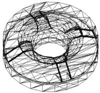
Using the Relief module you generate and process free-form surfaces, coin reliefs and shapes for engraving / milling applications. Here gridded relief data is processed in the relief format as ordered scatter plot. Relief data are built up similarly to the gridded printed design data such as PCX, BMP, TIFF … The Relief image consists of individual dots arranged in columns and lines, the pixels. Each pixel has a height value (Z information) assigned to it. In the various graphical representations this height information is drawn as colours, grey shades or curves. With this, a pixel is the smallest presentable element in the Relief. If intermediate points are required for projections, conversions or for milling, then these are interpolated The reliefs can be edited, scaled, filtered mirrored and converted into optimum milling tracks via various milling correction processes or employed as projection basis for the representation of 2D or 3D paths.
The Relief module supports, as extremely effective program, the areas:
- processing of reliefs, digitalised data, surface formats, photos (Relief).
- generation of reliefs from graphic elements (ReliefVTR).
- generation of milling data from relief (CAM) (Relief AutoCorr).
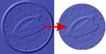
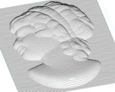
Point of emphasis for the relief format are artistic workpieces with many fine details and relatively flat characteristics (coin relief). Here lies the particular advantage of a simple and compact representation. Technical shaped parts have, on the other hand, rather uniform, in part, also very steep surfaces with few structures. For this surface descriptions (solids) are rather more suitable.
Some advantages and disadvantages of the processes:
| Surfaces (solids): |
Grid format: |
- With limited number of individual surfaces very compact data.
- The surface support points can be specified precisely.
- Depending on the CAD the surfaces can be freely edited.
|
- Simple representation of very fine artistic tasks.
- With many fine details a relatively compact relief is created.
- Digitalised data can be simply converted.
- Universal, rapid and exact milling correction processes for almost any desired tool shapes.
|
- Digitalised points have in part to be converted very laboriously via reverse engineering.
- Comprehensive tasks with very many details are, in practice, barely controllable.
- Milling offset calculations are, as a rule, limited on spheres.
|
- Surfaces must be gridded and can be passed on only with the accuracy of the grid resolution.
- Limitations with shapes with steep flanks.
- Because with equal grid resolution the relief data quantity with the dimensions increases immensely, the grid format restricts itself rather to smaller workpieces.
|
Exchange of vector data (paths) between relief and CAD.
If vector data (paths, contours, stretches, points) are required in the Relief module, then these are to be generated and marked in the CAD and are to be adopted in the relief module. In the relief module the paths marked in the CAD are shown in the colour greenish-blue. On the other hand paths, which have been generated in the relief module, after leaving the relief module, are adopted marked in the ActLayer. In the CAD, paths can be very easily drawn on the relief in the background after the option Relief has bee activated in the aid Graphic Background.
Aids in Relief.

 |
Graphic ZOOM +: enlarge image.
Frame a section of the image using a rectangle and present enlarged.
After clicking-on using , depending on the module, you obtain a zoom selection. |
 |
Graphic ZOOM -: reduce image.
Redraw the image at half size.
After clicking-on using , depending on the module, you obtain a zoom selection. |
 |
Graphic image NORM: image at set limits.
After clicking-on using you obtain a selection for graphic adjustment:
| Standard grey image: |
Adjust standard grey shades (colour) relief image. The colour table can be modified under Colours. The graphic indicator is activated by clicking-on Standard grey imaged and Adopt.. |
| Contrast dz-graphic: |
Relief plan view with accentuation of finer details. The contrast levels can be set in the range 1..5. |
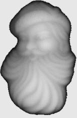
| Render: |
Display rendered the relief graphic with firmly fixed illumination source.
Standard setting. |
| Relief Object: |
Indication of the object limits (vector data). The display is switched ON and OFF by clicking-on. |
| Clipboard: |
Display of the vector data of the clipboard (,marked paths). The display is switched ON and OFF by clicking-on. |
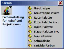
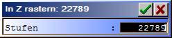
| Colour: |
Adjustment of the colour table for the relief image presentation. Various standard palettes are available (Grey stairs .. chocolate) and a free adjustment using variable colours. |
|
 |
New graphic image:
Redraw image with current settings. |
 |
All graphics:
Show ail graphic components (also outside the limits). |
 |
Input parameters (Program settings).
Current information can be found in the program help . |
 |
Help:
If you have questions on the operation, then please first use the integratedHelp.You can access Help also with already activated function using or using the aid ? Help and clock-on the function. |
 |
Selection ActLayer:
All operations are actioned using a layer of the ActLayer (current or active layer). The selected layer is selected here. |
Relief file menu.
Load and save relief data formats, images and CAD or digitiliser data in this menu. The functions in this menu always load only one complete relief and, with this, delete the previous relief content.
 Open relief. Open relief. |
Packed (.HRP) or unpacked relief data (.HRL) are loaded from a file in the working storage. For the differentiation of the data formats see Save Relief.
 Save Relief. Save Relief. |
Save the relief data in a file. To save you can select the two data types HRP and HRL.
| HRP |
The Relief is saved in packed format and with this requires less room on the data carrier. |
| HRL |
The relief is saved unpacked. This is, for example, required for data exchange with older programs and for further application, e.g. integration in ReliefVTR. |
 Import Relief . Import Relief . |
Foreign formats can be converted into a relief using Relief Import.
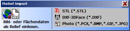
| Import STL.
|
STL is a stereo lithography format from the firm 3D-Systems. ASCII- and binary files are accepted for import. The measurement is always understood to be in mm. Advantage of STL is the clear definition and with this hardly any problems are to be expected with import. For good surface qualities you should pay attention that the surface is as highly resolved as possible and saved with small tolerances.
The STL data should as far as possible be available in the processing position. If this is not the case, then you can rotate the STL surfaces before generation of the relief. |
STL position:
The shape can be rotated about the X, Y and Z axes in the range -180°..+180°. Rotation takes place in 5° steps by clicking-on the buttons left and right alongside the angle indicators. Alternatively, the respective last rotated axis can also be rotated using the mouse thumb wheel. More accurate inputs are possible in the numeral field through manual input.
| Angle XY |
Horizontal rotation of the shape about the Z axis. |
| Angle YZ |
Rotation of the shape about the X axis. |
| Angle XZ |
Rotation of the shape about the Y axis.. |
| Volume aspect |
The graphic 3D display can be matched to the respective requirements. The following can be selected: the linear projection (vector graphic), relief projection, render projection or a combination of linear and relief or render projection. The projection shape shown in black is set. The blue listed projection shapes can be selected. Standard setting is linear + render projection. |
Following confirmation of the position the relief data is displayed/edited. As a rule the proposed values can be adopted unmodified. A modification of the data is recommended in individual cases only.
 |
Note: Depending on the quality of the surface generation, STL data can contain gaps (imperfections). These imperfections are mainly caused by the type of design (e.g. through the joining together of surface boundaries using arcs and segmented lines (polygons)). Small imperfections in the area of a relief point around a STL segment are closed automatically by the program. Larger imperfections. after an import, must be removed by filters or manually. A suitable filter for closing STL gaps is Correction Filter 2. |
| Zero point X0, Y0, Z0: |
Relief limit bottom left. By displacing the zero point in X/Y and enlarging the relief dimension, a border can, for example, be generated around the part. |
| Width (X), Height (H), Depth (Z): |
Relief dimensions. By displacing the zero point in X/Y and enlarging the relief dimension, a border can, for example, be generated around the part. |
| Resolution dx/dy: |
Grid resolution for the relief conversion. Smaller resolution values result in a larger relief data quantity and with this, longer calculation times. The proposed resolution, as a rule, surfaces for very fine work. |
Import DXF-3DFace.
Read-in of DXF data with 3DFACE surfaces. These data are, for example, generated using the Roland Picza digitalising machine.
Attention: Here only files with 3DFACE surfaces are read-in correctly-. Standard 2D or 3D DXF data are not suitable for this import and you obtain no result! In cases of doubt please check your data using a suitable editor or CAD.
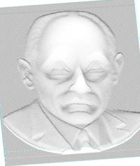
Import Photo.
Import a grey shade and adjust the dimension ( measurement). The program imports Bitmap data (256 grey shades = 8Bit grey shades = 1Byte/pixel) in the following formats:
| BMP |
Windows Bitmap with 256 grey shades. |
| gif |
CompuServ Bitmap with 256 grey shades. The gif -format contains no information on size or resolution. The image dimensions must be adjusted manually after import. |
| PCX |
Paintbrush Bitmap with 256 grey shades. |
| jpg, JPEG |
JPEG Bitmap with 256 grey shades, 8Bit colours and 24Bit colours. jpg images with 24Bit colours are converted into a grey shade image on import. |
A photo should be processed into a photostyler (e.g. Corel PHOTO-PAINT) before the milling path calculation and saved as grey shade image (8Bit/pixel – not in colour, exception .jpg). Images in .jpg format can also be saved as colour images (24Bit). These are converted into grey shade images on import.
Gridded photos (e.g. from journals/magazines) posses a very rough surface and should as far as possible be avoided or reworked into a suitable photostyler beforehand. Gridded images can also be improved using approximate finely/strongly.
The formats BMP, PCX, jpg and JPEG are imported already with the correct image dimensions. You can adjust the measurements in the following input. gif images have no resolution or image dimensions- These images must always be adjusted correctly. The relief Status is also displayed as check for the input of the relief dimensions .
| Proportional [Y/N]: |
With the setting YES all axes are also adjusted proportionately at the same time. The height – width – depth ratio remains the same. With the setting No the axes X/Y/Z can be determined individually. |
| Dimension XY/Z [mm]: |
Relief dimensions in the axes X/Y/Z. |
 Export relief. Export relief. |
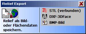 |
Convert and save the current relief in various foreign formats. |
STL (incorporated):
STL is a stereo lithography surface format of the firm 3D-Systems. For export STL binary files are created. Export processes with increased surface number. The surface is formed through adjoining triangular surfaces and is closed free of gaps. The max. permissible deviation to the relief is determined through the input tolerance. A large tolerance results in compact data with few STL surfaces, but large deviations to the relief. A small tolerance results in extensive data with many STL surfaces but also no deviations to the relief. The tolerance should not be selected too fine, because the therewith resultant surface number exceeds the potential of many target systems (CAD/ CAD). Tolerances < 0.01 mm should not be selected. For large relief enlargements the tolerance should lie significantly above this (0.05 .. 0.5 mm).
DXF-3DFace:
Export of the current relief into a DXF file using 3DFACE surfaces. This file can, for example, be read-in using AutoCAD. The surface is formed through adjoining rectangular surfaces. The max. permissible deviation to the relief is determined through the input tolerance. A large tolerance results in compact data with few STL surfaces, but large deviations to the relief. A small tolerance results in extensive data with many STL surfaces but also no deviations to the relief. The tolerance should not be selected too fine, because the therewith resultant surface number exceeds the potential of many target systems. Tolerances < 0.01 mm should not be selected. For large relief enlargements the tolerance should lie significantly above this (0.05 .. 0.5 mm).
BMP image:
Save the relief as grey shade image (256 shades) in BMP format.
 Status. Status. |
Indicate characteristics and dimensions of the relief file. The Z coordinates process positively upwards (opposite direction to LG1 format).
| File size [kB] : |
Size of the file in kByte. |
| Dimensions X*Y*Z [pix] : |
Measurement of the relief in dots. |
| Enlargement X*Y*Z [mm] : |
Enlargement of the relief in mm. |
| Left below X*Y*Z [mm] : |
Relief limit bottom left. |
| Right above X*Y*Z [mm] : |
Relief limit top right. |
| Scaling X,Y,Z : |
Scaling factor for X, Y and Z. |
| (Name) : |
Original name of the relief |
Export of relief extracts.
The functions in this menu always load only one complete relief and, with this, overwrite the previous content of the working storage. If a relief or part of a relief is to be imported to an existing relief, then this can take place using ReliefVTR . Input relief. In many cases the relief to be imported must be prepared for this purpose. For example, if the r is to be with any desired contour and not limited to rectangular. Using Input relief fundamentally all unpacked reliefs (.HRL) can be imported. The relief may not be packed for input. Extracts from reliefs are generated using the following functions Export extract and Export frame.
 Export extract. Export extract. |
Generate a rectangular or ellipse shaped extract from the current relief. The extract can be exported in a file or adopted as current relief. The relief extract is first limited by the two values, zero position and end position. The extract can be further limited in the following selection.
| Limits: |
A rectangular or an ellispe-shaped extract can be generated. |
| Width, height: |
Input of the desired width/height of the extract. |
| x0 left, y0 below, x1 right, y1 above: |
Positions of a boundary rectangle for the extract. |
| Dimensions in: |
There are three settings available for indication of numerals and position input:
| mm, Pt centre: |
Dimensions in mm, relief point centre. |
| mm, Pt external: |
Dimensions in mm, relief point external limit |
| Pix.: |
Dimensions in relief dots. |
|
| Export file: |
The extract is saved in a file. |
| Replace act. relief: |
The current (active) relief is replaced by the extract. |
 Export frame. Export frame. |
An extract from a relief, which lies within one or more frame contours, is exported. The parts of the relief which lie outside the frame contour, are faded out (do not overwrite the existing relief on importing). The frame is to be designed and marked in the CAD beforehand.
Procedure for export frame.
| 1 |
In the CAD draw one/several boundary contours. For this you can place the relief in the background using the aid Graphic background. |
| 2 |
Mark the boundary contours and change into the relief module. |
| 3 |
Select relief File . Export frame and the boundary contours. |
| 4 |
Save the relief limited using the boundary contour in a file. |
 Modify frame. Modify frame. |
 |
Edit the relief limits (clip or expand relief). |
| Extract XY: |
Create a relief extract. The area of the image to be framed by a rectangle is adopted and the rest is removed. For easier input of the boundary rectangle you can draw help lines beforehand in CAD. |
| Add border: |
Create an additional image border. A border in the specified width is inserted around the relief.
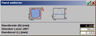
| Border width: |
Width of the border which is to be added to the relief. |
| Same Level Y/N: |
| YES: |
For the border the outermost pixel is duplicated outwards. |
| No: |
The height of the border is determined using Border level. |
|
| Border level (L): |
Height of the borders with Same level = No. |
|
| Limit above/ below: |
Limits the relief in Z (cut off relief top/bottom). For Z value input, first select a suitable (Z) point using the cursor in the relief. The Z level can be corrected to the desired value in the subsequent input. Capable of input are only values between minimum and maximum relief Z values. Following confirmation the relief is appropriately limited. |
 Scale. Scale. |
 |
Ein Relief in Größe und Auflösung anpassen. |
| Scale % |
Adjust size in X/Y/Z (input in %). Change of the scaling between 1% and 10000%. Values of 1%..99.999% reduce the image, Values 100,001%..10000% enlarge the image. With Proportional = YES all axes are the same, with No the axes are input individually. |
| Dimensions XYZ: |
Height-width ratio (input in mm). With Proportional = YES all axes are the same, with No the axes are input individually. |
| Reduce %: |
The image data are coarsened, i.e. image dots (pixels are removed and thus the resolution and the amount of data are reduced. Image data are modified through this function!
Dimension XY: Coarsening value 1%..99.999% |
| Reduce mm: |
The image data are coarsened, i.e. image dots (pixels are removed and thus the resolution and the amount of data are reduced. Image data are modified through this function!
Dimension XY: Coarsening value only smaller than the indicated value. |
| Grade: |
Coarsen grey tone (colour) grading: the grey tone table is converted to another grading. This function is only sensible for a coarsening of the grey steps.
Display grid in Z: display the grey tone grades.
Input shades: new number of grey tone shades. |
| Double resolution.: |
Double resolution of the complete image in X/Y. The position and enlargement remain unchanged. |
 Adjust limits. Adjust limits. |
 |
Match the relief to the working limits or working limits to the relief. |
| Max. graphic: |
Match image frame to graphic. The image limits are so adjusted that the graphic fills the complete image. |
| Centre graphic: |
Centre the graphic within the limits. The graphic is arranged centrally within the image frame. |
| Centre frame: |
Centre graphic an limits. The graphic frame and the graphic are so displaced that the centre of the frame lies at the point X = 0 and Y = 0. |
| Displace: |
Displace graphic. The relief is displaced using the cursor. With this a frame is also moved. Using the key the relief is adopted at the momentary position, using the key the function is aborted without an adoption. |
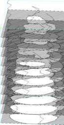
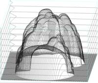
 Norm projection. Norm projection. |
The relief can be displayed in 3D in several versions.
- The type of presentation (gratings, vectors, dots or surfaces) is selected with the topmost buttons.
- The viewing direction is displayed schematically by means of a cuboid. You can adjust the direction by clicking-on the direction arrow in steps of 10 degrees using the cursor.
- Using PosnA adjust the line depiction colour. With PosnA without colour the perspective display takes place with adjustable height level marking.
- Following the graphic is drawn, aborts the input.
Zoom projection.
For display of a section (Zoom) select Zoom projection. The selected section is defined, using the cursor, through the two extreme positions of a rectangle (zero position and end position). One after the other both positions are input using the cursor. A position is confirmed with the key . If the key is operated, then the function is aborted and the image remains in its original condition. Following confirmation of the end position the image is deleted and the projection drawn anew enlarged. Before Zoom projection the image must have been adjusted using Norm projection.
Edit Relief menu.
 Layer edge. Layer edge. |
Scan of boundary lines for a selected Z level relief. The lines are determined as vector data. Following the selection ABSOLUTE/relative, a point is selected in the relief at the desired height.
 |
 |
 |
| Adjust layer edge |
Absolute height representation |
Relative height representation. |
| ABSOLUTE: |
Scan all contours at a height display. |
| Relative: |
Scan all contours at a gradient acclivity. For this the relief is converted temporarily into a height representation using relative acclivities. |
The level at which the boundary lines are scanned, must be selected beforehand using the cursor. The coordinates in X/Y/Z for this are displayed in the input line. In the following editing the level can be corrected or adjusted upwards or downwards.
 |
 |
 |
| Adjustment for layer edge. |
Relief section at level height. |
Relief using the traced contour. |
| Thicken: |
Thicken the traced contours up to max. 10 times relief resolution (pixel). |
| Level: |
Limiting height for the edge scan. The level can be edited in the range from min .. max (display above). For orientation a b/w image with the momentary limit set is also drawn at the same time. |
 Filter. Filter. |
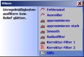 |
You can rework the relief and achieve flatter surfaces and/or filter out irregularities using the filter functions. Filters are mostly required for import data, e.g. import of dot clouds: Digitalising imperfections must be removed (error pixs, outliers, approximate). Or following import of STL data: gaps must be frequently be evened out (correction filter 2). The filters can also be called up several times for a stronger effect. |
| Error pixels: |
Individual dots are filtered. This has an impact only locally within a radius of one image dot, i.e. no appreciable change of quality though smoothing of the surface.
Max imperfection (0.01..10mm): The image dot (pixel), whose value deviates from its neighbouring dots by more than the specified max imperfection, is approximated (adjusted). An image edge of 1 pixel is not processed. |
| Outliers: |
The function outlier is the special surfaces filter for the removal of individual intensely different image dots (outliers) independent of their value. This filter has an impact only locally within a radius of one image dot, i.e. no appreciable change of quality though smoothing of the surface. |
| Approximate (strongly): |
The image contours or shapes are smoothed through approximate and approximate strongly . Approximate can, depending on requirement, be carried out several times. |
| Smooth: |
The relief resolution is doubled and, at the same time, the relief slightly smoothed. This filter produces significantly higher data quantities and should therefore be used for coarse images only. Reliefs with too high a resolution can be reduced again using scale . reduce (e.g.: [%] = 50). |
| Radius filter: |
Smooth the relief, all edges are rounded off. |
| Correction filter 1: |
Smooth the relief, all edges are rounded one-sided. |
| Correction filter 2: |
This filter fills gaps (e.g. following STL import) up to a
max. max width 2*Ir.
| Imperfection radius (Ir): |
Half of gap width to be filled. |
| Fill (flat/circular): |
Gap flat ,fill, spheroidally. |
| Type of calculation (exact/pointed): |
| Exact: |
Complex and error-free calculation. |
| Pointed: |
Rapid calculation for lightly curved surfaces.. |
|
|
 Mirror+ rotate. Mirror+ rotate. |
 |
Mirror the complete relief in X, Y, Z or rotate by +90 degrees / -90 degrees. |
| Mirror X/Y/Z: |
The relief is mirrored about the selected axis. |
| Counterblock XZ: |
Concurrent mirroring for a counterblock in X and Z direction. |
| Rotate +90°/-90°: |
The relief is rotated by +90°/-90°. |
|